Sentinel-1 InSAR Product Guide

This document is a guide for users of Interferometric Synthetic Aperture Radar (InSAR) Sentinel-1 products generated by the Alaska Satellite Facility (ASF). Users can request InSAR products On Demand in ASF's Vertex data portal, or make use of our HyP3 Python SDK or API.

This process requires Sentinel-1 IW SLC products as input. Input pairs can be selected in Vertex using either the Baseline Tool or the SBAS Tool search interfaces.

For a step-by-step tutorial on ordering On-Demand InSAR Products using Vertex, visit our InSAR On Demand! StoryMap. To learn more about the files included in the On Demand InSAR product packages and how to work with them, refer to our Exploring Sentinel-1 InSAR StoryMap.

InSAR processing requires a Digital Elevation Model (DEM) for the removal of topographic phase. We use the GLO-30 Copernicus DEM when processing our On Demand InSAR products. Refer to the Prepare the DEM File section for more information.

Coverage gaps in Copernicus DEM GLO-30 filled using GLO-90

The Copernicus DEM GLO-30 dataset does not provide coverage over Armenia and Azerbaijan. In the past, we have not supported InSAR product generation over those areas, due to the lack of DEM coverage. We now use the Copernicus DEM GLO-90 to fill those gaps.

The GLO-90 dataset has a pixel spacing of 90 meters, which is not as detailed as the 30-m pixel spacing in the GLO-30 DEM, but it does allow us to provide InSAR products in these regions, where they were previously unavailable.

ASF also offers burst-based Sentinel-1 InSAR products. This on-demand processing option allows users to submit InSAR jobs for individual SLC bursts rather than the full Sentinel-1 IW SLC products. Refer to our Sentinel-1 Burst InSAR Product Guide for more information on this option.

Users are cautioned to read the sections on limitations and error sources in InSAR products before attempting to use InSAR data. For a more complete description of the properties of SAR, see our Introduction to SAR guide.

Introduction

Interferometric Synthetic Aperture Radar (InSAR) processing uses two SAR images collected over the same area to determine geometric properties of the surface. Missions such as Sentinel-1 are designed for monitoring surface deformation using InSAR, which is optimal when acquisitions are made from a consistent location in space (short perpendicular baseline) over regular time intervals.

The phase measurements of two SAR images acquired at different times from the same place in orbit are differenced to detect and quantify surface changes, such as deformation caused by earthquakes, volcanoes, or groundwater subsidence.

InSAR can also be used to generate digital elevation models, but the optimal mission for DEM generation has the opposite characteristics of the Sentinel-1 mission. Topography is best mapped when the two acquisitions are obtained as close together as possible in time (short temporal baseline), but from different vantage points in space (larger perpendicular baseline than would be optimal for deformation mapping).

Brief Overview of InSAR

SAR is an active sensor that transmits pulses and listens for echoes. These echoes are recorded in phase and amplitude, with the phase being used to determine the distance from the sensor to the target and the amplitude yielding information about the roughness and dielectric constant of that target.

Figure 1: Two passes of an imaging SAR taken at time T₀ and T₀ + ∆t, will give two distances to the ground, R₁ and R₂. A difference between R₁ and R₂ shows motion on the ground. In this case, a subsidence makes R₂ greater than R₁. Credit: TRE ALTAMIRA

InSAR exploits the phase difference between two SAR images to create an interferogram that shows where the phase and, therefore, the distance to the target has changed from one pass to the next, as illustrated in Figure 1. There are several factors that influence the interferogram, including earth curvature, topographic effects, atmospheric delays, surface motion, and noise. With proper processing, Sentinel-1 InSAR can be used to detect changes in the earth's surface down to the centimeter scale. Applications include volcanic deformation, subsidence, landslide detection, and earthquake assessment.

Wavelengths

The SAR sensors on the Sentinel-1 satellites transmit C-band signals, with a wavelength of 5.6 cm. The signal wavelength impacts the penetration capability of the signal, so it is important to be aware of the sensor wavelength when working with SAR datasets. C-band SAR will penetrate more deeply into canopy or surfaces than an X-band signal, but not nearly as deep as an L-band SAR signal, which, with a wavelength on the order of 25 cm, is better able to penetrate canopy and return signals from the forest floor.

Different wavelengths are also sensitive to different levels of deformation. To detect very small changes over relatively short periods of time, you may require a signal with a smaller wavelength (such as X-band). However, signals with shorter wavelengths are also more prone to decorrelation due to small changes in surface conditions such as vegetation growth.

For slower processes that require a longer time interval to detect movement, longer wavelengths (such as L-band) may be necessary. C-band sits in the middle. It can detect fairly small changes over fairly short periods of time, but is not as sensitive to small changes as X-band or as able to monitor surface dynamics under canopy as L-band.

Polarizations

Polarization refers to the direction of travel of an electromagnetic wave. A horizontal wave is transmitted so that it oscillates in a plane parallel to the surface imaged, while a vertical wave oscillates in a plane perpendicular to the surface imaged.

Most modern SAR systems can transmit chirps with either a horizontal or vertical polarization. In addition, some of these sensors can listen for either horizontal or vertical backscatter. This gives rise to 4 different types of returns: HH, HV, VV, and VH, with the first letter indicating the transmission method and the second the receive method. For example, VH is a vertically polarized transmit signal with horizontally polarized echoes recorded.

For InSAR applications, processing is generally performed on the co-pol (VV or HH) data and not on the cross-pol (VH or HV) data. Also, each image used in an InSAR pair is required to be the same polarization - two HH images of the same area could form a valid pair, while a single HH with a single VV of the same area would not.

Baselines

Perpendicular Baseline

The term baseline refers to the physical distance between the two vantage points from which images used as an InSAR pair are acquired. The baseline is decomposed into perpendicular (also called normal) and parallel components, as shown in Figure 2.

To monitor surface deformation, the perpendicular baseline for the two acquisitions should be very small in order to maximize the coherence of the phase measurements.

In order to determine topography, two slightly different vantage points are required. Sensitivity to topography depends on the perpendicular baseline, the sensor wavelength, the distance between the satellite and the ground, and the sensor look angle.

Figure 2: Geometry of InSAR baselines. Two satellite passes image the same area on the ground from positions S₁ and S₂ , resulting in a baseline of B, which can be decomposed into perpendicular (B_⟂ ) and parallel (B_∥ ) components. Here Y is the direction of travel, referred to as the along-track or azimuth direction, and X is the direction perpendicular to motion, referred to as the cross-track or range direction. Credit: ASF

Temporal Baseline

In contrast to the (physical) baseline, the temporal baseline refers to the time separation between imaging passes. Along-track interferometry measures motion in the millisecond to second range. This technique can detect ocean currents and rapidly moving objects like boats. Differential interferometry is the standard method used to detect motion in the range of days to years. This is the type of interferometry that is performed by the Sentinel-1 HyP3 InSAR processing algorithm. Table 1 lists different temporal baselines, their common names, and what they can be used to measure.

Duration	Known as	Measurement of
ms to sec	along-track	ocean currents, moving object detection, MTI
days	differential	glacier/ice fields/lava flows, surface water extent, hydrology
days to years	differential	subsidence, seismic events, volcanic activity, crustal displacement

Table 1: Temporal baselines and what they measure. Different geophysical phenomena can be detected based upon the temporal baseline. In general, the longer the temporal baseline, the smaller the motion that can be detected.

Critical Baseline

Large baselines are better than small for topographic mapping. However, as the baseline increases, coherence decreases. At some point, it is impossible to create an interferogram because of baseline decorrelation. The maximum viable baseline per platform, referred to as the critical baseline, is a function of the distance to the ground, the wavelength, and the viewing geometry of the platform.

For Sentinel-1, this critical baseline is about 5 km. In practice, if the perpendicular baseline between images is more than 3/4 of the critical baseline, interferogram creation will be problematic due to the level of noise.

For deformation mapping, it is best to minimize the perpendicular baseline whenever possible, but there may be tradeoffs in terms of finding suitable temporal baselines. In most cases, however, pairs selected for deformation mapping will have perpendicular baselines much smaller than the critical baseline.

Ordering On Demand InSAR Products

All of ASF's On Demand InSAR products are generated using ASF's HyP3 platform. Jobs can be submitted for processing using the Vertex data portal, the HyP3 Python SDK or the HyP3 API.

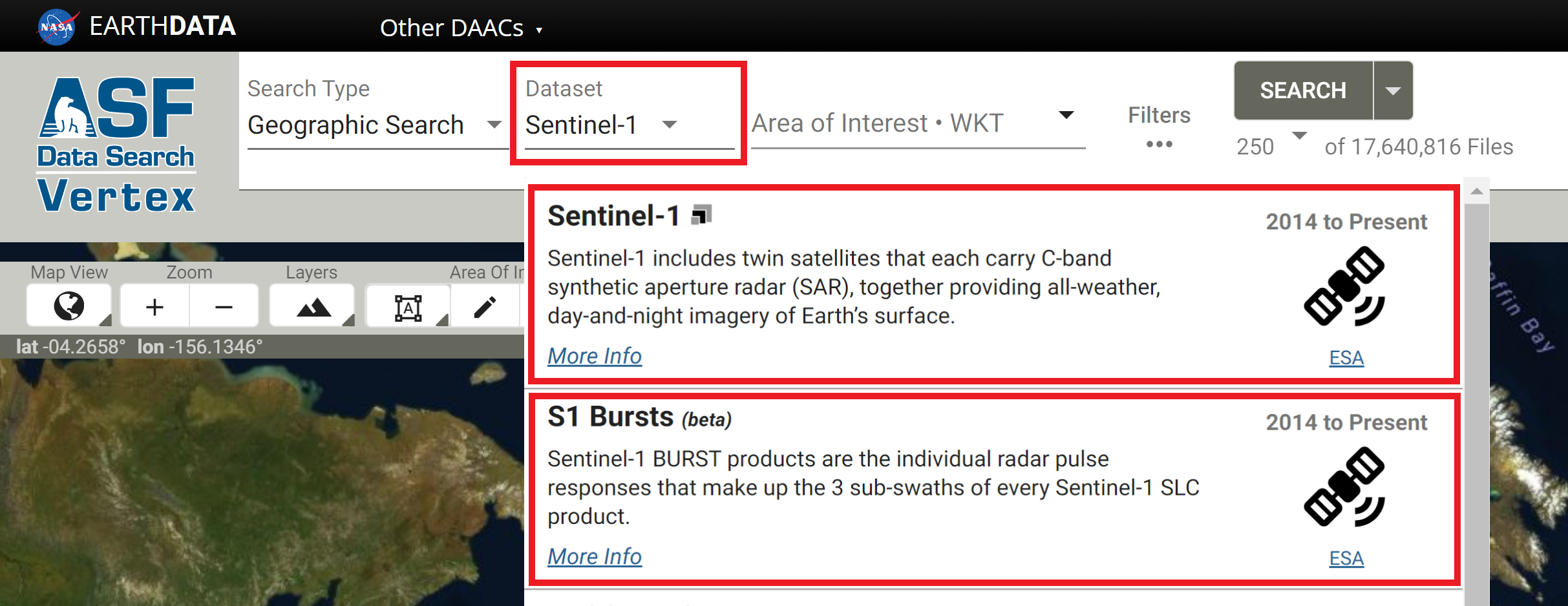
Vertex

InSAR pairs are selected in Vertex using either the Baseline Search or the SBAS Search interface. The process of selecting pairs is the same for both IW SLC products and individual SLC bursts, but you will need to select the appropriate dataset when searching for content. As illustrated below, select the Sentinel-1 option in the Dataset menu to search for IW SLC products, and select the S1 Bursts option to search for individual SLC bursts.

The Baseline tool is the best option for selecting specific InSAR pairs. Use the Geographic Search to find an image that covers your time and area of interest, select that item in the results, and click the Baseline button in the center panel. The Baseline tool then displays all of the scenes that could be used to generate an interferogram using the selected image. Scroll through the results to find pairs to add to the On Demand queue, or click on items displayed in the plot to highlight that particular image pair.

The SBAS tool is designed for generating time series of InSAR pairs. As with the Baseline search, you can launch the SBAS search from the center panel of a Geographic Search result. It will display all of the valid InSAR pairs through time based on the acquisition location of the input scene. This functionality is designed for processing a series of interferograms to be used in SBAS (Small BAseline Subset) analysis. The results can be adjusted based on baseline criteria (both perpendicular and temporal), and restricted to specific periods of time. Once the list is refined, you have the option to add all of the InSAR pairs displayed in the results to the On Demand queue.

HyP3 SDK and API

The HyP3 SDK and API provide support for creating interferograms based on a pair of selected granules. To identify granules you'd like to process, we suggest using the Geographic, Baseline and SBAS search tools in Vertex. If you'd prefer to request interferogram processing programmatically, we suggest using Vertex's companion Python package: asf_search. This HyP3 SDK Jupyter Notebook provides you with an example of how you can use the asf_search and hyp3_sdk packages together to identify and create stacks of InSAR products.

Considerations for Selecting an InSAR Pair

When selecting an InSAR pair, observe the following required conditions:

1. Images from an identical orbit direction (either ascending or descending)
2. Images with identical incidence angles and beam mode
3. Images with identical resolution and wavelength (usually from the same sensor)
4. Images with the same viewing geometry (same path and frame)
5. Images with identical polarizations (both HH or VV)

In addition, the following suggestions may be helpful:

1. Use images from similar seasons/growth/weather conditions
2. For deformation mapping: limited spatial separation of acquisition locations (small physical baseline)
3. For topographic mapping: limited time separation between images (small temporal baseline)

To analyze deformation caused by a single discrete event, such as an earthquake, select images that bracket the event as closely in time as possible. Keeping the window narrowly focused on the time of the event will reduce the impacts of other processes that may mask the signal of the event of interest.

Processing Options and Optional Files

There are several options users can set when ordering InSAR On Demand products, including setting some processing parameters and selecting additional files to include in the output product package.

New: Adaptive Phase Filter parameter is now customizable!

There is now an option to adjust the adaptive phase filter parameter value when submitting On Demand InSAR jobs. This option is available in Vertex, as well as in the HyP3 API and Python SDK! Refer to the Adaptive Phase Filter section for more information.

Processing Options

When submitting jobs for processing, there are a number of parameters that can be set by the user.

Number of Looks

The number of looks drives the resolution and pixel spacing of the output products. Selecting 10x2 looks will yield larger products with 80 m resolution and pixel spacing of 40 m. Selecting 20x4 looks reduces the resolution to 160 m and reduces the size of the products (roughly 1/4 the size of 10x2 look products), with a pixel spacing of 80 m. The default is 20x4 looks.

Adaptive Phase Filter

When ordering InSAR On Demand products, users can choose to set a custom value for the Goldstein-Werner adaptive phase filter (adf). This filter improves fringe visibility and reduces phase noise in interferograms, particularly for InSAR pairs with low coherence. The filter impacts both wrapped and unwrapped interferograms, as well as the optional displacement maps generated from the unwrapped interferogram.

Users can set the adaptive phase filter parameter (𝛼) value within the range of 0 to 1, with 0 indicating that no filtering occurs, and 1 indicating the strongest level of filtering. The default value is 0.6. The value should generally be greater than 0.2, and interferograms with very low coherence will benefit from higher values (closer to 1). Setting this value to 0 will result in no filter being applied.

The filter is applied adaptively, meaning that regions with high coherence (where fringe patterns are easily discernible) will have more smoothing applied, while regions with low coherence will undergo less smoothing, so as not to remove residues that may represent actual deformation signals. Using this filter approach allows more of the interferogram to be unwrapped. For more information, refer to Goldstein and Werner's 1998 paper, Radar interferogram filtering for geophysical applications.

Apply Water Mask

There is an option to apply a water mask. This mask includes coastal waters and most inland waterbodies. Masking waterbodies can have a significant impact during the phase unwrapping, as water can sometimes exhibit enough coherence between acquisitions to allow for unwrapping to occur over waterbodies, which is invalid.

A GeoTIFF of the water mask is always included with the InSAR product package, but when this option is selected, the conditional water mask will be applied along with coherence and intensity thresholds during the phase unwrapping process. Water masking is turned off by default.

The water mask is generated by ASF using data from OpenStreetMap and/or ESA WorldCover depending on location. Areas within Canada, Alaska, and Russia are primarily covered by ESA WorldCover data, while the rest of the world is covered by OpenStreetMap data. Refer to the Water Masking documentation page for more details.

This water mask is available for all longitudes, but data is only available from -85 to 85 degrees latitude. All areas between 85 and 90 degrees north latitude are treated as water, and all areas between 85 and 90 degrees south latitude are treated as land for the purposes of the water mask.

Water masks were previously generated from the Global Self-consistent, Hierarchical, High-resolution Geography Database (GSHHG) dataset, but we transitioned to using the OpenStreetMap/ESA WorldCover datasets in February 2024 to improve performance. In addition to being a more recent and accurate dataset, this also allows us to mask most inland waterbodies. When using the GSHHG dataset, we only masked large inland waterbodies; with the new mask, all but the smallest inland waterbodies are masked.

We originally applied a 3 km buffer on coastlines and a 5 km buffer on the shorelines of inland waterbodies in the water mask dataset before using it to mask the interferograms, in an effort to reduce the chance that valid land pixels would be excluded from phase unwrapping. It appears, however, that the inclusion of more water pixels is more detrimental to phase unwrapping than the exclusion of some land pixels, so as of September 27, 2022, the water mask used for this option is no longer buffered.

Visit our InSAR Water Masking Tutorial for more information about how different water masking approaches can impact the quality of an interferogram.

Optional Files

In addition to the processing options, users can choose to add a number of ancillary files to the product package. These files are not included by default, as they increase the size of the product package and may not be of interest to all users.

In Vertex, check the box in the "Include" section of the options to add these optional files to the product package. When using the HyP3 API or SDK, set the parameter to true.

1. The look vectors are stored in two files. The look vector refers the look direction back towards the sensor. The lv_theta (θ) indicates the SAR look vector elevation angle at each pixel, ranging from -π/2 (down) to π/2 (up). The look vector elevation angle is defined as the angle between the horizontal surface and the look vector with positive angles indicating sensor positions above the surface. The lv_phi (φ) map indicates the SAR look vector orientation angle at each pixel, ranging from -π (west) to π (west). The look vector orientation angle is defined as the angle between the East direction and the projection of the look vector on the horizontal surface plane. The orientation angle increases towards north, with the North direction corresponding to π/2 (and south to -π/2). Both angles are expressed in radians. The default is to not include these files in the output product bundle.

2. The displacement maps convert the phase difference values from the unwrapped interferogram into measurements of ground displacement in meters. The line-of-sight displacement map indicates the amount of movement away from or towards the sensor. The vertical displacement calculates the vertical component of the line-of-sight displacement, using the assumption that all deformation is in the vertical direction. These files are excluded from the product package by default.

3. The wrapped phase GeoTIFF can be included in the output package. The browse version of this GeoTIFF (_color_phase.png) is always included, but the GeoTIFF version is not included by default. The specific color ramp displayed in the png is most valuable for many users, but some may wish to work with the actual wrapped phase values.

4. The incidence angle maps indicate the angle of the radar signal. The local incidence angle is defined as the angle between the incident radar signal and the local surface normal, expressed in radians, while the ellipsoid incidence angle indicates the angle between the incident radar beam and the direction perpendicular to the WGS84 ellipsoid model. These files are excluded from the product package by default.

5. A copy of the DEM used for processing can optionally be included in the product package. The file has been projected to a UTM Zone coordinate system, and pixel values indicate the elevation in meters. The elevation values will differ from the original Copernicus DEM GLO-30 dataset, as a geoid correction has been applied. The source DEM is also downsampled to twice the pixel spacing of the output product to smooth it for use in processing, then resampled again to match the pixel spacing of the InSAR product. The DEM is excluded by default.

InSAR Workflow

The InSAR workflow used in HyP3 was developed by ASF using GAMMA software. The steps include pre-processing steps, interferogram preparation, and product creation. Once these steps are performed, an output product package will be created. See product packaging for details on the individual files included in the package.

Pre-Processing

Pre-processing steps prepare the SAR images to be used in interferometry. The pre-processing steps include image selection, ingest (including calibration), creation of a suitable DEM, and calculation of the burst overlap.

Select an InSAR Pair

Although it is possible to start from RAW data, Sentinel-1 InSAR processing is typically done using Interferometric Wide swath Single Look Complex (IW SLC) data as the input. This means that the data has been formed into an image through SAR processing, but has not been multi-looked.

The SLC pair is defined by the user, either through the Vertex interface, or using the HyP3 API or SDK. To ensure consistency, the older SLC image is always used as the reference image, and the younger SLC image is always used as the secondary image. This means that positive values in the resulting unwrapped interferogram represent movement away from the SAR platform and negative values represent movement towards the SAR platform. However, these values are relative to the reference point of the unwrapped interferogram. See the phase unwrapping section for more details.

Ingest SLC data into GAMMA format

Once the InSAR pair has been identified, the selected SLC data are ingested into GAMMA internal format. This is performed by the GAMMA program par_s1_slc. GAMMA format has raw data files (only data, no headers or line leaders) with metadata stored in external files with a .par extension.

During ingest into GAMMA's internal format, the SLC data is calibrated by applying the calibration coefficients that are supplied with each product. This process puts the SAR backscatter into a known scale where the diffuse volume scattering of the Amazon rainforest is a constant -6.5 dB.

Immediately after ingesting the SLC, the state vectors are updated to use the best available state vectors. The state vector types in order of absolute correctness are original predicted (O), restituted (R), and precision (P). In practice, one will never receive an InSAR product that uses the original predicted orbit - only granules for which a restituted or precision orbit is available can be used in HyP3 InSAR processing. The orbit type used for generating the InSAR product is indicated in the product filename, as shown in Figure 3.

Figure 3: Position of the orbit type in the HyP3 product name.

Prepare the DEM File

In order to create differential InSAR products that show motion on the ground, one must subtract the topographic phase from the interferogram. The topographic phase, in this case, is replicated by using an existing DEM to calculate the actual topographic phase. This phase is then removed from the interferogram leaving just the motion or deformation signal (plus atmospheric delays and noise).

The DEM that is used for HyP3 InSAR processing is the 2022 Release of the Copernicus GLO-30 Public DEM dataset publicly available on AWS. For more information about the 2022 updates, see the 'Releases' section of this article.

The Copernicus DEM provides higher-quality products over a wider area than the older DEMs (SRTM and NED) previously used to generate ASF's On Demand products. Refer to our Digital Elevation Model Documentation for more information. The Copernicus DEM provides global coverage at 30-m pixel spacing, except for areas over Armenia and Azerbaijan. These gaps in coverage are filled with the Copernicus GLO-90 Public DEM, which has 90-m pixel spacing.

The DEM tiles necessary to cover the input granules for the InSAR product are downloaded. A geoid correction is applied to the DEM, and it is resampled to match the output resolution of the InSAR product (160 m for 20x4 products, 80 m for 10x2 products) and projected to the appropriate UTM Zone for the granule location.

Calculate Overlapping Bursts

The IW SLC Sentinel-1 data comes in three sub-swaths. However, a further subdivision is made in the data, wherein bursts occur. Bursts are the fundamental building block for Sentinel-1 imagery. Each one is a portion of the final image, around 1500 lines long and one sub-swath width wide. Thus, the more busts, the longer the file is in length.

Each burst is precisely timed to repeat at a given time interval. This consistent repeat combined with precise velocity control gives rise to the fact that the bursts start at the same time on each pass around the globe.

For example, a burst images a piece of the Galápagos Islands. The next time that same piece of the island is imaged, the time of day will be the same, to within few milliseconds. Only the frames containing overlapping bursts can be used to perform InSAR processing. This means that if there is no burst overlap in the pair selected as input, the InSAR process will not run.

Repeatable burst timing is exploited by HyP3 in order to calculate the bursts that overlap between two scenes. These overlapping bursts are the only ones used in the rest of the InSAR process. The rest are discarded.

Interferogram Creation, Co-registration and Refinement

Before the interferogram is created, the lookup table that maps from the SLC image space into a ground range image space is created. At this time, the interferogram of the topography is simulated using the previously prepared DEM.

Once these steps have been performed, the two SLCs are co-registered to within 0.02 pixels. This is done by iteratively using the following steps:

1. Resample the secondary SLC using previously calculated offset polynomial
2. Match the reference and secondary SLC images using intensity cross-correlation
3. Estimate range and azimuth offset polynomial coefficients from results of matching
4. Create a differential interferogram using the co-registered SLCs and the simulated interferogram
5. Update offset polynomial by adding the current estimates

Note that these steps are automatically run 4 times. At that point, if the last offset calculated was more than 0.02 pixels, then the procedure will fail to complete.

Provided the images passed the check for convergence, the next co-registration step employs the Enhanced Spectral Diversity (ESD) algorithm to match the two scenes to better than 1/100th of a pixel. This is accomplished by examining the overlap area between subsequent bursts. If there is even a small offset, the phase between the bursts will not match. This phase mismatch is then used to calculate the corresponding azimuth offset.

To finish interferogram processing, steps 1 through 4 are run once again, this time with the offsets from the ESD included. The output of this entire process is a wrapped interferogram.

Phase Unwrapping

All of the phase differences in wrapped interferograms lie between -π and π. Phase unwrapping attempts to assign multiples of 2π to add to each pixel in the interferogram to restrict the number of 2π jumps in the phase to the regions where they may actually occur. These regions are areas of radar layover or areas of deformation exceeding half a wavelength in the sensor's line of sight. Thermal noise and interferometric decorrelation can also result in these 2π phase discontinuities called residues.

The phase unwrapping algorithm used for these products is Minimum Cost Flow (MCF) and Triangulation. Refer to this Technical Report from GAMMA Remote Sensing for more information on the MCF phase unwrapping approach.

Filtering

Before the interferogram can be unwrapped, it must be filtered to remove noise. This is accomplished using an adaptive spectral filtering algorithm. This adaptive interferogram filtering aims to reduce phase noise, increase the accuracy of the interferometric phase, and reduce the number of interferogram residues as an aid to phase unwrapping. In this case, residues are points in the interferogram where the sum of the phase differences between pixels around a closed path is not 0.0, which indicates a jump in phase.

Masking

Another step before unwrapping is to create a validity mask to guide the phase unwrapping process. This mask is generated by applying thresholds to the coherence and/or amplitude (backscatter intensity) values for an image pair. For On Demand InSAR products, we set the amplitude threshold to be 0.0 (in power scale), so that data is only excluded based on the coherence threshold.

Coherence is estimated from the normalized interferogram. The pixel values in this file range from 0.0 (total decorrelation) to 1.0 (perfectly coherent). Any input pixel with a coherence value less than 0.1 is given a validity mask value of zero and not used during unwrapping.

Change to Validity Mask Thresholds

In the past, we also used an amplitude threshold of 0.2 (in power scale) when generating the validity mask. While this approach tends to mask out inland waters, providing a less noisy interferogram in some cases, it also masks arid regions that have low amplitude values but reasonably high coherence. As of March 2022, we have set the amplitude threshold to 0.0, so that coherence is the only driver of the validity mask.

In some cases, pixels over water may still meet the coherence threshold criteria for inclusion, even though they are not valid for use during phase unwrapping. When the water masking option is applied, the validity mask is further amended to apply 0 values to any pixels classified as water in the water mask.

When processing scenes with extensive coverage by coastal waters or large inland waterbodies, there can be erroneous deformation signals or phase jumps introduced if unwrapping proceeds over water as if it were land. In such cases, choosing the option to apply the water mask can significantly improve the results. Refer to our InSAR Water Masking Tutorial for more information.

Reference point

In order to perform phase unwrapping, a reference point must be selected. The unwrapping will proceed relative to this reference point; the 2π integer multiples will be applied to the wrapped phase using this pixel as the starting point. The unwrapped phase value is set to 0 at the reference point.

Ideally, the reference point for phase unwrapping would be located in an area with high coherence in a stable region close to an area with surface deformation. Choosing an optimal reference point requires knowledge of the site characteristics and examination of the interferogram, which is not practical in an automated, global workflow.

By default, ASF's On Demand InSAR products use the location of the pixel with the highest coherence value as the reference point. The coherence map is examined to determine the maximum value, and all pixels with this value are examined using a 9-pixel window. The pixel with the highest sum of values within its 9-pixel window is selected as the reference point. If more than one pixel has the same 9-pixel sum, the pixel closest to the origin pixel (bottom left corner for ascending scenes, top right corner for descending scenes) is selected.

This may be an appropriate reference point location in many cases, as it meets the criteria of having high coherence, and stable areas have higher coherence than areas undergoing significant deformation. If a user wants to set a different location as the phase unwrapping reference point, however, a correction can be applied to the unwrapped interferogram.

For more information on the impact of the phase unwrapping reference point location on unwrapped phase and displacement measurements, refer to the Limitations section of this document, which also includes instructions for applying a correction based on a custom reference point.

Geocoding and Product Creation

After the phase is unwrapped, the final steps are geocoding and product creation.

Geocoding

Geocoding is the process of reprojecting pixels from SAR slant range space (where all the calculations have been performed) into map-projected ground range space (where analysis of products is simplest). Using the look up table previously computed, this process takes each pixel in the input product and relocates it to the UTM zone of the DEM used in processing. This is accomplished using nearest-neighbor resampling so that original pixel values are preserved.

Product Creation

Files are next exported from GAMMA internal format into the widely-used GeoTIFF format, complete with geolocation information. GeoTIFFs are created for amplitude, coherence, and unwrapped phase by default, and a water mask GeoTIFF is also included in the product package. Optionally, GeoTIFFs of wrapped phase, look vectors, displacement maps (line-of-sight and vertical), and incidence angle maps can be included, as can a copy of the DEM used for processing.

Product Packaging

HyP3 InSAR output is a zip file containing various files, including GeoTIFFs, PNG browse images with geolocation information, Google Earth KMZ files, a metadata file, and a README file.

Naming Convention

The InSAR product names are packed with information pertaining to the processing of the data, presented in the following order, as illustrated in Figure 4.

• The platform names, either Sentinel-1A or Sentinel-1B, are abbreviated "A" or "B", indicating the reference and secondary granule's imaging platform
• The reference start date and time and the secondary start date and time, with the date and time separated by the letter T
• The polarizations for the pair, either HH or VV, the orbit type, and the days of separation for the pair
• The product type (always INT for InSAR) and the pixel spacing, which will be either 80 or 40, based upon the number of looks selected when the job was submitted for processing
• The software package used for processing is always GAMMA for GAMMA InSAR products
• User-defined options are denoted by three characters indicating whether the product is water masked (w) or not (u), the scene is clipped (e for entire area, c for clipped), and whether a single sub-swath was processed or the entire granule (either 1, 2, 3, or F for full swath)
  • Currently, only the water masking is available as a user-selected option; the products always include the full granule extent with all three sub-swaths
• The filename ends with the ASF product ID, a 4 digit hexadecimal number

Figure 4: Breakdown of ASF InSAR naming scheme.

Image Files

All of the main InSAR product files are 32-bit floating-point single-band GeoTIFFs. To learn more about the rasters included in the product package, refer to the Exploring Sentinel-1 InSAR StoryMap tutorial.

• The amplitude image is the calibrated radiometric backscatter from the reference granule in sigma-nought power. The image is terrain corrected using a geometric correction, but not radiometrically corrected.
• The coherence file pixel values range from 0.0 to 1.0, with 0.0 being completely non-coherent and 1.0 being perfectly coherent.
• The unwrapped phase file shows the results of the phase unwrapping process. Negative values indicate movement towards the sensor, and positive values indicate movement away from the sensor. This is the main interferogram output.
• The wrapped phase file indicates the interferogram phase after applying the adaptive filter immediately before unwrapping. Values range from negative pi to positive pi. (optional)
• The line-of-sight displacement file indicates the displacement in meters along the look direction of the sensor. The sign is opposite to that of the unwrapped phase: positive values indicate motion towards the sensor and negative values indicate motion away from the sensor. (optional)
• The vertical displacement is generated from the line of sight displacement values, and makes the assumption that deformation only occurs in the vertical direction. Note that this assumption may not hold true in cases where the deformation also has a horizontal component. Positive values indicate uplift, and negative values indicate subsidence. (optional)
• The look vectors theta (θ) and phi (φ) describe the elevation and orientation angles of the sensor's look direction. (optional)
• The incidence angle maps indicate the angle between the incident signal and the surface normal of either the terrain (local incidence angle) or the ellipsoid (ellipsoid incidence angle). (optional)
• The DEM file gives the local terrain heights in meters, with a geoid correction applied. (optional)
• The water mask file indicates coastal waters and most inland waterbodies. Pixel values of 1 indicate land and 0 indicate water. This file is in 8-bit unsigned integer format.

If the water mask option is selected, the water mask is applied prior to phase unwrapping to exclude water pixels from the process. The water mask is generated using the OpenStreetMap and ESA WorldCover datasets. Refer to the Water Masking Processing Option section and our InSAR Water Masking Tutorial for more information about water masking.

Browse images are included for the wrapped (color_phase) and unwrapped (unw_phase) phase files, which are in PNG format and are each 2048 pixels wide. The browse images are displayed using a cyclic color ramp to generate fringes.

• Each fringe in a wrapped (color_phase) browse image represents a 2-pi phase difference, and the line-of-sight displacement for each fringe is equivalent to half the wavelength of the sensor. The wavelength of Sentinel-1 is about 5.6 cm, so each 2-pi fringe represents a line-of-sight displacement of about 2.8 cm.
• Each fringe in an unwrapped (unw_phase) browse image represents a phase difference of 6 pi. Because each 2-pi difference is equivalent to half the wavelength of the sensor, each 6-pi fringe represents about 8.3 cm of line-of-sight displacement for these Sentinel-1 products.

KMZ files are included for the wrapped (color_phase) and unwrapped (unw_phase) phase images, which allow users to view the outputs in Google Earth or other platforms that support kmz files.

The tags and extensions used and example file names for each raster are listed in Table 2 below.

Extension	Description	Example
_amp.tif	Amplitude	S1AB_20171111T150004_20171117T145926_VVP006_INT80_G_ueF_4D09_amp.tif
_corr.tif	Normalized coherence file	S1AB_20171111T150004_20171117T145926_VVP006_INT80_G_ueF_4D09_corr.tif
_unw_phase.tif	Unwrapped geocoded interferogram	S1AB_20171111T150004_20171117T145926_VVP006_INT80_G_ueF_4D09_unw_phase.tif
_wrapped_phase.tif	Wrapped geocoded interferogram	S1AB_20171111T150004_20171117T145926_VVP006_INT80_G_ueF_4D09_wrapped_phase.tif
_los_disp.tif	Line-of-sight displacement	S1AB_20171111T150004_20171117T145926_VVP006_INT80_G_ueF_4D09_los_disp.tif
_vert_disp.tif	Vertical displacement	S1AB_20171111T150004_20171117T145926_VVP006_INT80_G_ueF_4D09_vert_disp.tif
_lv_phi.tif	Look vector φ (orientation)	S1AB_20171111T150004_20171117T145926_VVP006_INT80_G_ueF_4D09_lv_phi.tif
_lv_theta.tif	Look vector θ (elevation)	S1AB_20171111T150004_20171117T145926_VVP006_INT80_G_ueF_4D09_lv_theta.tif
_dem.tif	Digital elevation model	S1AB_20171111T150004_20171117T145926_VVP006_INT80_G_ueF_4D09_dem.tif
_inc_map_ell.tif	Ellipsoid incidence angle	S1AB_20171111T150004_20171117T145926_VVP006_INT80_G_ueF_4D09_inc_map_ell.tif
_inc_map.tif	Local incidence angle	S1AB_20171111T150004_20171117T145926_VVP006_INT80_G_ueF_4D09_inc_map.tif
_water_mask.tif	Water mask	S1AB_20171111T150004_20171117T145926_VVP006_INT80_G_ueF_4D09_water_mask.tif
_color_phase.kmz	Wrapped phase kmz file	S1AB_20171111T150004_20171117T145926_VVP006_INT80_G_ueF_4D09_color_phase.kmz
_unw_phase.kmz	Unwrapped phase kmz file	S1AB_20171111T150004_20171117T145926_VVP006_INT80_G_ueF_4D09_unw_phase.kmz
_color_phase.png	Wrapped phase browse image	S1AB_20171111T150004_20171117T145926_VVP006_INT80_G_ueF_4D09_color_phase.png
_unw_phase.png	Unwrapped phase browse image	S1AB_20171111T150004_20171117T145926_VVP006_INT80_G_ueF_4D09_unw_phase.png

Table 2: Image files in product package

Metadata Files

The product package also includes a number of metadata files.

Extension	Description	Example
.README.md.txt	Main README file for GAMMA InSAR	S1AB_20171111T150004_20171117T145926_VVP006_INT80_G_ueF_4D09.README.md.txt
.txt	Parameters and metadata for the InSAR pair	S1AB_20171111T150004_20171117T145926_VVP006_INT80_G_ueF_4D09.txt
.tif.xml	ArcGIS compliant XML metadata for GeoTIFF files	S1AB_20171111T150004_20171117T145926_VVP006_INT80_G_ueF_4D09_unw_phase.tif.xml
.png.xml	ArcGIS compliant XML metadata for PNG files	S1AB_20171111T150004_20171117T145926_VVP006_INT80_G_ueF_4D09_color_phase.png.xml
.png.aux.xml	Geolocation information for png browse images	S1AB_20171111T150004_20171117T145926_VVP006_INT80_G_ueF_4D09_color_phase.png.aux.xml

Table 3: Metadata files in product package

README File

The text file with extension .README.md.txt explains the files included in the folder, and is customized to reflect that particular product. Users unfamiliar with InSAR products should start by reading this README file, which will give some background on each of the files included in the product folder.

InSAR Parameter File

The text file with extension .txt includes processing parameters used to generate the InSAR product as well as metadata attributes for the InSAR pair. These are detailed in Table 4.

Name	Description	Possible Value
Reference Granule	ESA granule name for reference scene (of the two scenes in the pair, the dataset with the oldest timestamp)	S1A_IW_SLC__1SDV_20200116T032559_20200116T032627_030820_038928_F5DC
Secondary Granule	ESA granule name for secondary scene (of the two scenes in the pair, the dataset with the newest timestamp)	S1B_IW_SLC__1SDV_20200128T032559_20200128T032627_030995_038F51_7D4F
Reference Pass Direction	Orbit direction of the reference scene	DESCENDING
Reference Orbit Number	Absolute orbit number of the reference scene	30741
Secondary Pass Direction	Orbit direction of the reference scene	DESCENDING
Secondary Orbit Number	Absolute orbit number of the secondary scene	31091
Baseline	Perpendicular baseline in meters	58.3898
UTCTime	Time in the UTC time zone in seconds	12360.691361
Heading	Spacecraft heading measured in degrees clockwise from north	193.2939317
Spacecraft height	Height in meters of the spacecraft above nadir point	700618.6318999995
Earth radius at nadir	Ellipsoidal earth radius in meters at the point directly below the satellite	6370250.0667
Slant range near	Distance in meters from satellite to nearest point imaged	799517.4338
Slant range center	Distance in meters from satellite to the center point imaged	879794.1404
Slant range far	Distance in meters from satellite to farthest point imaged	960070.8469
Range looks	Number of looks taken in the range direction	20
Azimuth looks	Number of looks taken in the azimuth direction	4
InSAR phase filter	Name of the phase filter used	adf
Phase filter parameter	Dampening factor	0.6
Resolution of output (m)	Pixel spacing in meters for output products	80
Range bandpass filter	Range bandpass filter applied	no
Azimuth bandpass filter	Azimuth bandpass filter applied	no
DEM source	DEM used in processing	GLO-30
DEM resolution	Pixel spacing in meters for DEM used to process this scene	160
Unwrapping type	Phase unwrapping algorithm used	mcf
Phase at Reference Point	Original unwrapped phase value at the reference point (set to 0 in output unwrapped phase raster)	-4.21967
Azimuth line of the reference point in SAR space	Row number (in SAR space) of the reference point	2737.0
Range pixel of the reference point in SAR space	Column number (in SAR space) of the reference point	739.0
Y coordinate of the reference point in the map projection	Latitude of the reference point in projected coordinates (UTM Zone - meters)	4112453.3223
X coordinate of the reference point in the map projection	Longitude of the reference point in projected coordinates (UTM Zone - meters)	589307.6248
Latitude of the reference point (WGS84)	Latitude of the reference point in WGS84 Geographic Coordinate System (degrees)	37.1542125
Longitude of the reference point (WGS84)	Longitude of the reference point in WGS84 Geographic Coordinate System (degrees)	40.00574707
Unwrapping threshold	Minimum coherence required to unwrap a given pixel	none
Speckle filter	Speckle filter applied	no

Table 4: List of InSAR parameters included in the parameter text file

ArcGIS-Compatible XML Files

There is an ArcGIS-compatible XML file for each raster in the product folder. When ArcGIS Desktop users view any of the rasters in ArcCatalog or the Catalog window in ArcMap, they can open the Item Description to view the contents of the associated XML file. ArcGIS Pro users can access the information from the Metadata tab. These files will not appear as separate items in ArcCatalog, though if you use Windows Explorer to look at the contents of the folder you will see them listed individually. Because each one is named identically to the product it describes (with the addition of the .xml extension), ArcGIS recognizes the appropriate file as the raster’s associated metadata, and integrates the metadata accordingly.

ArcGIS users should take care not to change these XML files outside of the ArcGIS environment; changing the filename or content directly may render the files unreadable by ArcGIS.

Those not using ArcGIS will still find the contents of these XML files useful, but will have to contend with the XML tagging when viewing the files as text or in a browser.

Auxiliary Geolocation Files

Geolocation XML files (aux files) are included for each of the PNG browse images to allow for proper display in GIS platforms.

Limitations

Baseline Calculation

The baseline is defined as the difference of the platform positions when a given area is imaged. HyP3 baselines are calculated using the best state vectors available. If precise orbits are not yet available for the input granules, restituted orbits will be used. The original predicted orbits are not used for InSAR processing in HyP3. If no restituted or precise state vectors are available, the process will not run.

Coherence

The phase measurements in the two images used in InSAR must be coherent in order to detect change. Random changes in phase from one acquisition to the next can mask actual surface deformation. Vegetation is a common driver of decorrelation, as changes can easily take place in the interval between two acquisitions due to growth, seasonal changes, or wind effects. It will be difficult to generate valid interferograms with C-band data in heavily vegetated regions due to lack of coherence even with fairly short time intervals.

Consider seasonality when selecting image pairs. Decorrelation can be particularly high when comparing phase from different seasons. Changes in the condition of vegetation (especially deciduous canopies), snow, moisture, or freeze/thaw state can impact phase measurements. In cases where a temporal baseline is required that spans seasons, it may be better to use an annual interferogram if possible so that the images are more comparable in terms of seasonality.

Line-of-Sight Measurements

When looking at a single interferogram, the deformation measurements in the line-of-sight orientation of the sensor indicate relative motion towards or away from the sensor. InSAR is not sensitive to motion in the azimuth direction of the satellite, so motion that occurs in the same direction as the satellite's direction of travel will not be detected.

A single interferogram cannot be used to determine the relative contributions of vertical and horizontal movement to the line-of-sight displacement measurement. The vertical displacement map is generated based on the assumption that the movement is entirely in the vertical direction, which may not be realistic for some processes. To determine how much of the signal is driven by vertical vs. horizontal movement, you must either use a time series of interferograms, or use reference measurements with known vertical and horizontal components (such as GNSS measurements from the region of deformation) to deconstruct the line-of-sight displacement.

All displacement values are calculated relative to a reference point, which may or may not be an appropriate benchmark for measuring particular areas of displacement within the interferogram.

Phase Unwrapping Reference Point

The reference point for phase unwrapping is set to be the location of the pixel with the highest coherence value. As described in the phase unwrapping section, this may not always be an ideal location to use as a reference point. If it is located in an area undergoing deformation, or in a patch of coherent pixels that is separated from the area undergoing deformation by a gap of incoherent pixels, the unwrapping may be of lower quality than if the reference point was in a more suitable location.

Even when there are not phase unwrapping errors introduced by phase discontinuities, it is important to be aware that unwrapped phase differences and displacement values are all calculated relative to the reference point. The phase difference value of the reference point is set to 0 during phase unwrapping, so any displacement values will be relative to that benchmark. If the location of the default reference point is in the middle of an area that underwent deformation, displacement values may be different than expected.

If you are interested in the amount of displacement in a particular area, you may wish to choose your own reference point. The ideal reference point would be in an area of high coherence beyond where deformation has occurred. The unwrapped phase measurements can be adjusted to be relative to this new reference point, and displacement values can be recalculated accordingly. To adjust the values in the unwrapped phase GeoTIFF, simply select a reference point that is optimal for your use case and subtract the unwrapped phase value of that reference point from each pixel in the unwrapped phase raster:

ΔΨ^* = ΔΨ - Δψ_ref

where ΔΨ^* is the adjusted unwrapped phase, ΔΨ is the original unwrapped phase, and Δψ_ref is the unwrapped phase value at the new reference point.

Impacts on Displacement Measurements

The measurements in the displacement maps are calculated from the unwrapped phase values, so will similarly be impacted by the location of the reference point. You may wish to recalculate the displacement values relative to a new reference point. The approach for correcting the displacement maps will be different for the line-of-sight and vertical measurements.

Correcting Line-of-Sight Displacement Maps

If you have already corrected the unwrapped phase raster, you can calculate a new line-of-sight (LOS) displacement map by applying the following calculation on a pixel-by-pixel basis using the unwrapped phase GeoTIFF:

ΔΩ^* = - ΔΨ^* λ / 4π

where ΔΩ^* is the adjusted line-of-sight displacement in meters, ΔΨ^* is the adjusted unwrapped phase, and λ is the wavelength of the sensor in meters (0.055465763 for Sentinel-1).

Setting the ΔΨ^* value to be negative reverses the sign so that the difference is relative to the earth rather than the sensor. A positive phase difference value indicates subsidence, which is unintuitive when thinking about movement on the earth's surface. Applying the negative will return positive displacement values for uplift and negative values for subsidence.

If you are not interested in adjusted unwrapped phase values, you can also directly correct the LOS Displacement map included optionally in the InSAR product package:

ΔΩ^* = ΔΩ - Δω_ref

where ΔΩ^* is the adjusted line-of-sight displacement in meters, ΔΩ is the original line-of-sight displacement in meters, and Δω_ref is the line-of-sight displacement value at the new reference point.

Correcting Vertical Displacement Maps

Vertical displacement maps cannot be adjusted directly, and must be recalculated from the adjusted unwrapped phase image. You will also need the θ look vector map (lv_theta GeoTIFF) for this calculation. The look vector maps are not included in the InSAR product package by default; the option to Include Look Vectors must be selected when ordering the product.

To calculate an adjusted vertical displacement raster, calculate the adjusted unwrapped phase, then apply the following:

Δϒ^* = - ΔΨ^* λ cos(½π - LV_θ) / 4π

where Δϒ^* is the adjusted vertical displacement in meters, ΔΨ^* is the adjusted unwrapped phase, λ is the wavelength of the sensor in meters (0.055465763 for Sentinel-1), and LV_θ is the theta look vector (from the lv_theta GeoTIFF).

As with the LOS Displacement maps, setting the ΔΨ^* value to be negative reverses the sign so that the difference is relative to the earth rather than the sensor. Applying the negative will return positive displacement values for uplift and negative values for subsidence.

Displacement Values from a Single Interferogram

In general, calculating displacement values from a single interferogram is not recommended. While the displacement rasters provided with ASF's On Demand InSAR products can be helpful in visualizing changes, we do not recommend that you rely on a single interferogram when coming to conclusions about surface displacement, even if you apply a correction based on a manually selected reference point. It will be more robust to use a time series approach to more accurately determine the pattern of movement. When using SAR time-series software such as MintPy, you have the option to select a specific reference point, and the values of the input rasters will be adjusted accordingly.

Error Sources

On Demand InSAR products do not currently correct for some common sources of error in interferometry, such as atmospheric effects. Further processing or time series analysis can be performed by the user to identify or reduce the impact of some of these errors when using On Demand InSAR products for analysis.

Atmospheric Delay

While SAR signals can penetrate clouds, atmospheric conditions can delay the transmission of the signal. This results in phase differences that can look like surface deformation signals but are actually driven by differences in the atmospheric conditions between the pair of acquisitions used to generate the interferogram.

In some cases, atmospheric errors can be corrected by using an atmospheric model to remove the impacts of the turbulent delay from the interferogram. Another approach is to use time series analysis to identify outliers.

Always doubt your interferogram first! View the interferogram critically, and consider if fringe patterns could potentially be driven by atmospheric effects. In general, it is best to avoid drawing conclusions from the outcome of a single interferogram.

Tropospheric phase may be less impactful when considering small-scale deformation. As such, if you are using ASF's Sentinel-1 Burst InSAR products to look at deformation signals that are smaller than 1 km², you should consider using methods other than the typical atmospheric model-based corrections to remove the effects of atmospheric delay. Potential methods in this case include applying band-pass or high-pass spatial filters, or spatial averaging filters such as the approach outlined in Bekaert et al., 2020.

Turbulent Delay

These delays are generally caused by differences in water vapor distribution from one image to the next. They often manifest as wobbly or sausage-shaped fringes, and can potentially mask the signal of a small earthquake.

Stratified Delay

This type of delay is driven mostly by pressure and temperature differences or gradients through the atmospheric column, and often correlates with topography. This atmospheric signature can be confused with movement caused by volcanic activity. If there are multiple volcanoes in an image, and they all exhibit similar patterns, the signal is likely being driven by this type of atmospheric delay.

DEM Errors

A DEM is used to remove topographic phase impacts, but if there are inaccuracies in the DEM, residual impacts of those errors can remain in the interferogram.

Orbit Uncertainties

This is generally not an issue for Sentinel-1 data, as the orbits are very precise and generally reliable. On Demand InSAR products are only processed once restituted or precise orbits are available. Orbit uncertainties are more problematic when working with datasets from older missions.